Segregation
Contents
Segregation#
In brief#
Social segregation refers to the separation of groups on the grounds of personal or cultural traits. Separation can be physical (e.g., in schools or neighborhoods) or virtual (e.g., in social networks).
More in Detail#
Social segregation refers to the “separation of socially defined groups” [1]. People are partitioned into two or more groups on the grounds of personal or cultural traits that can foster discrimination, such as gender, age, ethnicity, income, skin color, language, religion, political opinion, membership of a national minority, etc. (see entry on Grounds of Discrimination). Contact, communication, or interaction among groups are limited by their physical, working or socio-economic distance. Such a separation is observed when dissecting the society into organizational units (neighborhoods, schools, job types).
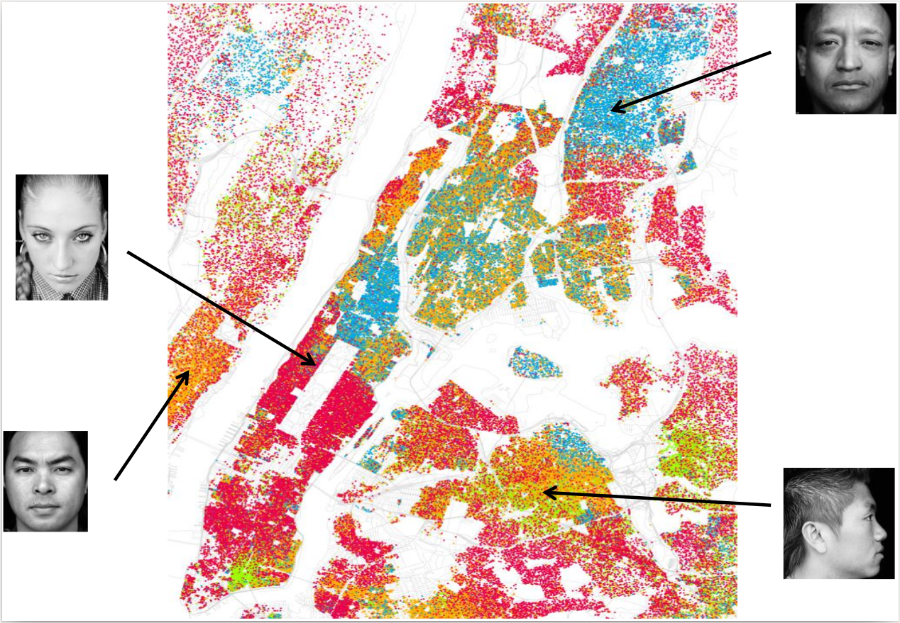
Fig. 17 Racial spatial segregation in New York City, based on Census 2000 data [2]. One dot for each 500 residents. Red dots are Whites, blue dots are Blacks, green dots are Asian, orange dots are Hispanic, and yellow dots are other races.#
Early studies on residential segregation trace back to 1930’s [3]. In this context, social groups are set apart in neighborhoods where they live in, in schools they attend to, or in companies they work at. As sharply pointed out in Fig. 17, racial segregation (a.k.a. residential segregation on the grounds of race) very often emerges in cities characterized by ethnic diversity. Schelling’s segregation model [4, 5] shows that there is a natural tendency to spatial segregation, as a collective phenomenon, even if each individual is relatively tolerant – in his famous abstract simulation model, Nobel laureate Schelling assumed that a person changes residence only if less than 30% of the neighbors are of his/her own race.
[6] argued that segregation is shifting from ancient forms on the grounds of racial, ethnic and gender traits to modern socio-economic and cultural segregation on the basis of income, job position, and political-religious opinions. An earlier comparison of ideological segregation of the American electorate online and offline is offered in [7]. The paper found that segregation in news consumption is higher online than offline, but significantly lower than the segregation of face-to-face interactions with neighbors, co-workers, or family members. More recently, it has been warned that the filter bubble generated by personalization of online social networks may foster segregation [8], opinion polarization [9], and lack of consensus between different social groups. Segregation in social network has been investigated in [10], with experiments on segregation on the grounds of sex and age for directors in the boards of the companies. Other works have focused on religious social networks [11],
A segregation index provides a quantitative measure of the degree of segregation of social groups (e.g., Blacks, Whites, Hispanics, etc.) distributed among units of social organization (e.g., schools, neighborhoods, jobs, etc.). Several indexes have been proposed in the literature. The surveys [12, 13] represent the earliest attempts to categorize them. Afterward, [14] provided a shared classification with reference to five key dimensions: evenness, exposure, concentration, centralization, and clustering. Finally, [15] adapts segregation measure to graphs representing social networks. In this entry, we will consider basic evenness and exposure indexes. Other three classes of indexes are specifically concerned with spatial notions of segregation. Concentration indexes measure the relative amount of physical space occupied by social groups in an urban area. Centralization indexes measure the degree to which a group is spatially located near the center of an urban area. Clustering indexes measure the degree to which group members live disproportionately in contiguous areas.
We restrict here to consider binary indexes, which assume a partitioning of the population into two groups, say majority and minority (but could be men/women, native/immigrant, White/NonWhite, etc.). Let \(T\) be size of the total population, \(0 < M < T\) be the size of the minority group, and \(P = M/T\) be the overall fraction of the minority group. Assume that there are \(n\) organizational units (or simply, units), and that for \(i \in [1, n]\), \(t_i\) is the size of the population in unit \(i\), \(m_i\) is the size of the minority group in unit \(i\), and \(p_i = m_i/t_i\) is the fraction of the minority population in unit \(i\).
Evenness indexes. Evenness indexes measure the difference in the
distributions of social groups among organizational units. The
dissimilarity index \(D\) is the weighted mean absolute deviation of
every unit’s minority proportion from the global minority proportion:
\(D = \frac{1}{2 \cdot P \cdot (1-P)} \sum_{i=1}^n \frac{t_i}{T}
\cdot | p_i - P | \label{equ:dissimilarity}\)
The normalization factor
\(2 \cdot P \cdot (1-P)\) is to obtain an index in the range \([0, 1]\).
Since \(D\) measures dispersion of minorities over the units, higher
values of the index mean higher segregation. Dissimilarity is minimum
when for all \(i \in [1, n]\), \(p_i = P\), namely the distribution of the
minority group is uniform over units. It is maximum when for all
\(i \in [1, n]\), either \(p_i = 1\) or \(p_i = 0\), namely every unit
includes members of only one group (complete segregation).
The second widely adopted index is the information index, also known
as the Theil index in social sciences [16] and normalized
mutual information in machine learning [17]. Let the
population entropy be \(E = -
P \cdot \log{P}-(1-P) \cdot \log{(1-P)}\), and the entropy of unit \(i\) be
\(E_i = - p_i \cdot \log{p_i}-(1-p_i) \cdot \log{(1-p_i)}\). The
information index is the weighted mean fractional deviation of every
unit’s entropy from the population entropy:
\(H = \sum_{i=1}^n \frac{t_i}{T} \cdot \frac{(E-E_i)}{E}\)
Information index ranges in \([0, 1]\). Since it denotes a relative reduction in
uncertainty in the distribution of groups after considering units,
higher values mean higher segregation of groups over the units.
Information index reaches the minimum when all the units respect the
global entropy (full integration), and the maximum when every unit
contains only one group (complete segregation).
The third evenness measure is the Gini index, defined as the mean
absolute difference between minority proportions weighted across all
pairs of units, and normalized to the maximum weighted mean difference.
In formula:
\(\label{eq:Gini}
G = \frac{1}{2 \cdot T^2 \cdot P \cdot (1-P)} \cdot \sum_{i=1}^n
\sum_{j=1}^n t_i \cdot t_j \cdot |p_i - p_j|\)
Here
\(\sum_{i=1}^n \sum_{j=1}^n t_i \cdot t_j \cdot |p_i - p_j|\) is the
weighted mean absolute difference. The normalization factor is obtained
by maximizing such a value. The definition of the Gini index stems from
econometrics, where it is used as a measure of the inequality of income
distribution [18]. The Gini index ranges in \([0, 1]\)
with higher values denoting higher segregation. The maximum and minimum
values are reached in the same cases of the dissimilarity index.
Exposure indexes. Exposure indexes measure the degree of potential
contact, or possibility of interaction, between members of social
groups. The most used measure of exposure is the isolation index
[19], defined as the likelihood that a member of the
minority group is exposed to another member of the same group in a unit.
For a unit \(i\), this can be estimated as the product of the likelihood
that a member of the minority group is in the unit (\(m_i/M\)) by the
likelihood that she is exposed to another minority member in the unit
(\(m_i/t_i\), or \(p_i\)) – assuming that the two events are independent.
In formula:
\(I = \frac{1}{M} \cdot \sum_{i=1}^n m_i \cdot p_i\)
The right hand-side formula can be read as the minority-weighted average of minority proportions in units. The isolation index ranges over \([P, 1]\), with higher values denoting higher segregation. The minimum value is reached when for \(i \in [1, n]\), \(p_i = P\), namely the distribution of the minority group is uniform over the units. The maximum value is reached when there is only one \(k \in [1, n]\) such that \(m_k = t_k = M\), namely there is a unit containing all minority members and no majority member.
A dual measure is the interaction index, which is the likelihood that
a member of the minority group is exposed to a member of the majority
group in a unit. By reasoning as above, this leads to the formula:
\(\mathit{Int} = \frac{1}{M} \cdot \sum_{i=1}^n m_i \cdot (1-p_i)\)
It clearly holds that \(I + \mathit{Int} = 1\). Hence, lower values denote
higher segregation. A more general definition of interaction index
occurs when more than two groups are considered in the analysis, so that
the exposure of the minority group to one of the other groups is worth
to be considered [14].
The key problem of assessing social segregation has been investigated by hypothesis testing, i.e., by formulating one or more possible contexts of segregation against a certain social group, and then in empirically testing such hypotheses. Such an approach is currently supported by statistical tools, such as the R packages OasisR1 and seg2 [20], or by GIS tools such as the Geo-Segregation Analyzer3 [21]. A tool for multidimensional exploration of segregation index has been proposed4 in [22].
Bibliography#
- 1
Douglas S Massey. Segregation and the perpetuation of disadvantage. In The Oxford Handbook of the Social Science of Poverty, pages 369–393. Oxford University Press, 2016.
- 2
Eric Fischer. Distribution of race and ethnicity in US major cities. 2011. under Creative Commons licence, CC BY-SA 2.0. URL: http://www.flickr.com/photos/walkingsf/sets/72157624812674967/detail/.
- 3
Nancy A Denton and Douglas S Massey. Residential segregation of Blacks, Hispanics, and Asians by socioeconomic status and generation. Social Science Quarterly, 69(4):797–817, 1988.
- 4
Thomas C Schelling. Dynamic models of segregation. Journal of Mathematical Sociology, 1(2):143–186, 1971.
- 5
W. A. V. Clark. Residential preferences and neighborhood racial segregation: a test of the Schelling segregation model. Demography, 28(1):1–19, 1991.
- 6
Douglas S. Massey, Jonathan Rothwell, and Thurston Domina. The changing bases of segregation in the United States. Annals of the American Academy of Political and Social Science, 626:74–90, 2009.
- 7
Matthew Gentzkow and Jesse M Shapiro. Ideological segregation online and offline. Quarterly Journal of Economics, 126(4):1799–1839, 2011.
- 8
Seth Flaxman, Sharad Goel, and Justin M Rao. Filter bubbles, echo chambers, and online news consumption. Public Opinion Quarterly, 80:298–320, 2016. URL: http://ssrn.com/abstract=2363701.
- 9
Michael Maes and Lukas Bischofberger. Will the personalization of online social networks foster opinion polarization? 2015. URL: http://ssrn.com/abstract=2553436.
- 10
Alessandro Baroni and Salvatore Ruggieri. Segregation discovery in a social network of companies. J. Intell. Inf. Syst., 51(1):71–96, 2018.
- 11
Jiantao Hu, Qian-Ming Zhang, and Tao Zhou. Segregation in religion networks. EPJ Data Sci., 8(1):6:1–6:11, 2019.
- 12
Otis Dudley Duncan and Beverly Duncan. A methodological analysis of segregation indexes. American Sociological Review, 20(2):210–217, 1955.
- 13
D. R. James and K. E. Tauber. Measures of segregation. Sociological Methodology, 13:1–32, 1985.
- 14(1,2)
Douglas S Massey and Nancy A Denton. The dimensions of residential segregation. Social Forces, 67(2):281–315, 1988.
- 15
Michal Bojanowski and Rense Corten. Measuring segregation in social networks. Soc. Networks, 39:14–32, 2014.
- 16
R. Mora and J. Ruiz-Castillo. Entropy-based segregation indices. Sociological Methodology, 41:159–194, 2011.
- 17
T. Mitchell. Machine Learning. The Mc-Graw-Hill Companies, Inc., 1997.
- 18
Joseph L Gastwirth. A general definition of the Lorenz curve. Econometrica: Journal of the Econometric Society, 39(6):1037–1039, 1971.
- 19
Wendell Bell. A probability model for the measurement of ecological segregation. Social Forces, 32(4):357–364, 1954.
- 20
Seong-Yun Hong, David O'Sullivan, and Yukio Sadahiro. Implementing spatial segregation measures in R. PLoS ONE, 9(11):e113767, 2014.
- 21
Philippe Apparicio, Joan Carles Martori, Amber L. Pearson, Éric Fournier, and Denis Apparicio. An open-source software for calculating indices of urban residential segregation. Social Science Computer Review, 32(1):117–128, 2014.
- 22
Alessandro Baroni and Salvatore Ruggieri. Scube: A tool for segregation discovery. In EDBT, 542–545. OpenProceedings.org, 2019.
This entry was readapted from Alessandro Baroni and Salvatore Ruggieri. Segregation discovery in a social network of companies. J. Intell. Inf. Syst., 51(1):71–96, 2018 by Salvatore Ruggieri